Decoding the Neuron’s Spark: Building Intuition for Action Potential Dynamics

Introduction

Ever wondered how your brain manages to tell your hand to grab that slice of pizza before your roommate does? It’s all thanks to an incredibly complex, yet surprisingly efficient communication network, your nervous system. Think of it as the internet of your body, but instead of cat videos and online shopping, it’s buzzing with urgent messages about survival (like pizza acquisition) and other important stuff, like not walking into walls.

This network relies on specialized cells called neurons, which are basically your body’s tiny gossips. They constantly chatter with each other, passing along information in the form of rapid electrical signals called action potentials (Drukarch and Wilhelmus 2023). These aren’t your grandma’s static shocks; they’re more like carefully crafted Morse code messages, zipping along neural pathways at impressive speeds. Imagine each neuron as a tiny town crier, shouting the latest news (or sensory input) to the next town over.

Now, you might be thinking, “Electrical signals? Sounds complicated.” And you’d be right. But fear not! In this post, we’re going to break down the magic behind action potentials using a simplified mathematical model. Think of it as a cheat sheet for understanding how these tiny electrical storms work. We’ll start with the basics and gradually add complexity, like adding extra gossip to the town crier’s message, until we have a decent understanding of the dynamics at play. No PhD in neuroscience required (though a craving for pizza is always helpful). So, buckle up, because we’re about to drive into the electrifying world of neuronal communication!

Photo from Encyclopaedia Britannica

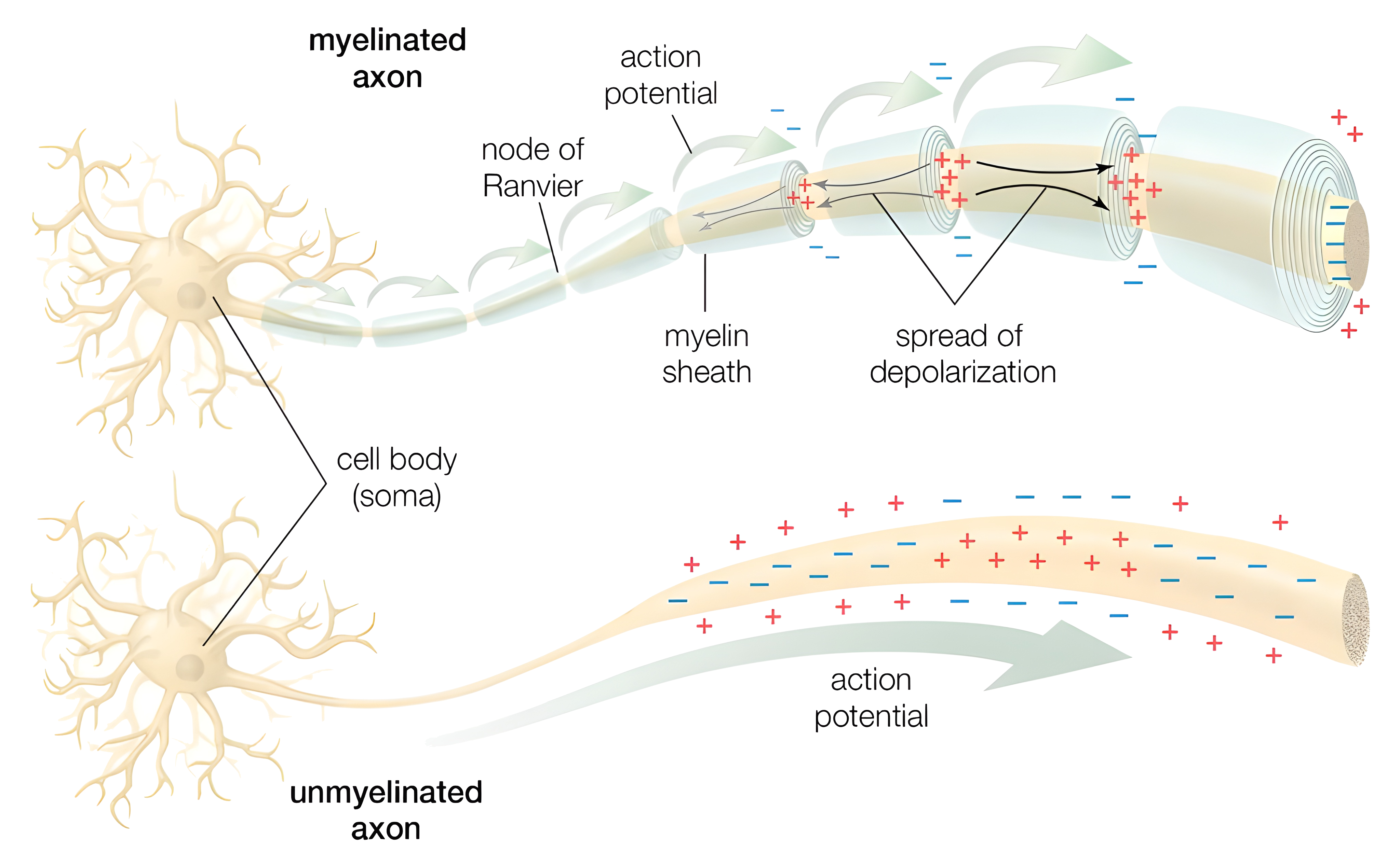
The Neuron as a Simple Circuit: A First Approximation

Let’s imagine our neuron not as a bustling town crier, but as a tiny, slightly bored house. It’s got walls (the cell membrane), an inside (intracellular fluid), and an outside (extracellular fluid). These fluids are salty solutions, full of charged particles called ions like sodium, potassium, and chloride (the electrolyte gang you see advertised in sports drinks). Now, because these fluids have different concentrations of these ions, there’s a difference in electrical charge between the inside and the outside of the house. This difference in charge is what we call the membrane potential, measured in millivolts (mV). Think of it like a tiny battery inside the neuron, just waiting to be used.

Normally, this “battery” sits at a resting voltage of around -70 mV. Why negative? It’s just a convention: we define the outside of the cell as zero, and the inside is negatively charged relative to it. So, our little neuron house is just chilling, with a slight negative charge inside (like a grumpy teenager refusing to get out of bed).

Now, our neuron’s walls (the membrane) aren’t completely airtight. They have tiny holes, called leak channels, which allow some ions to slowly trickle in and out. It’s like having a slightly leaky faucet, not a major flood, but a constant drip. These leaks are crucial because they maintain that resting membrane potential (Rubin 2021).

Photo from Neuroscience: Canadian 1st Edition

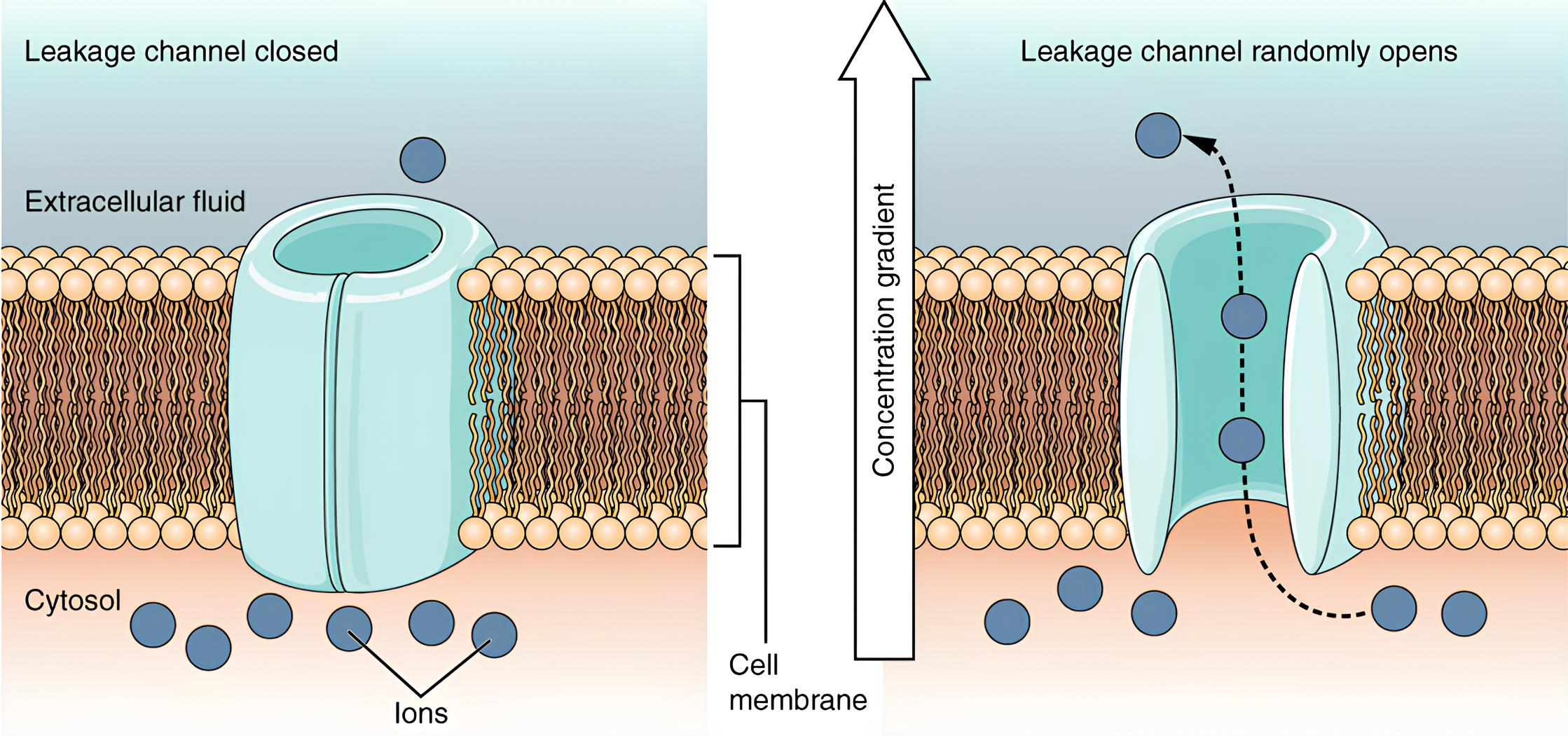
Another important property of the membrane is its ability to store electrical charge, much like a capacitor in an electronic circuit. This is called capacitance. Imagine the membrane as two conductive plates (the inside and outside of the cell) separated by an insulator (the membrane itself). When there’s a difference in charge across the membrane (our membrane potential), it stores some of that charge (Rubin 2021). It’s like a tiny electrical reservoir, ready to release its charge when needed.

So, to summarize our lazy neuron house:

• Membrane potential: A voltage difference between the inside and outside.
• Leak channels: Tiny holes that allow ions to slowly leak across the membrane, maintaining the resting potential.
• Capacitance: The membrane’s ability to store electrical charge.

Expanding our Intuition Using Math: Waking Up the Sleeping Neuron

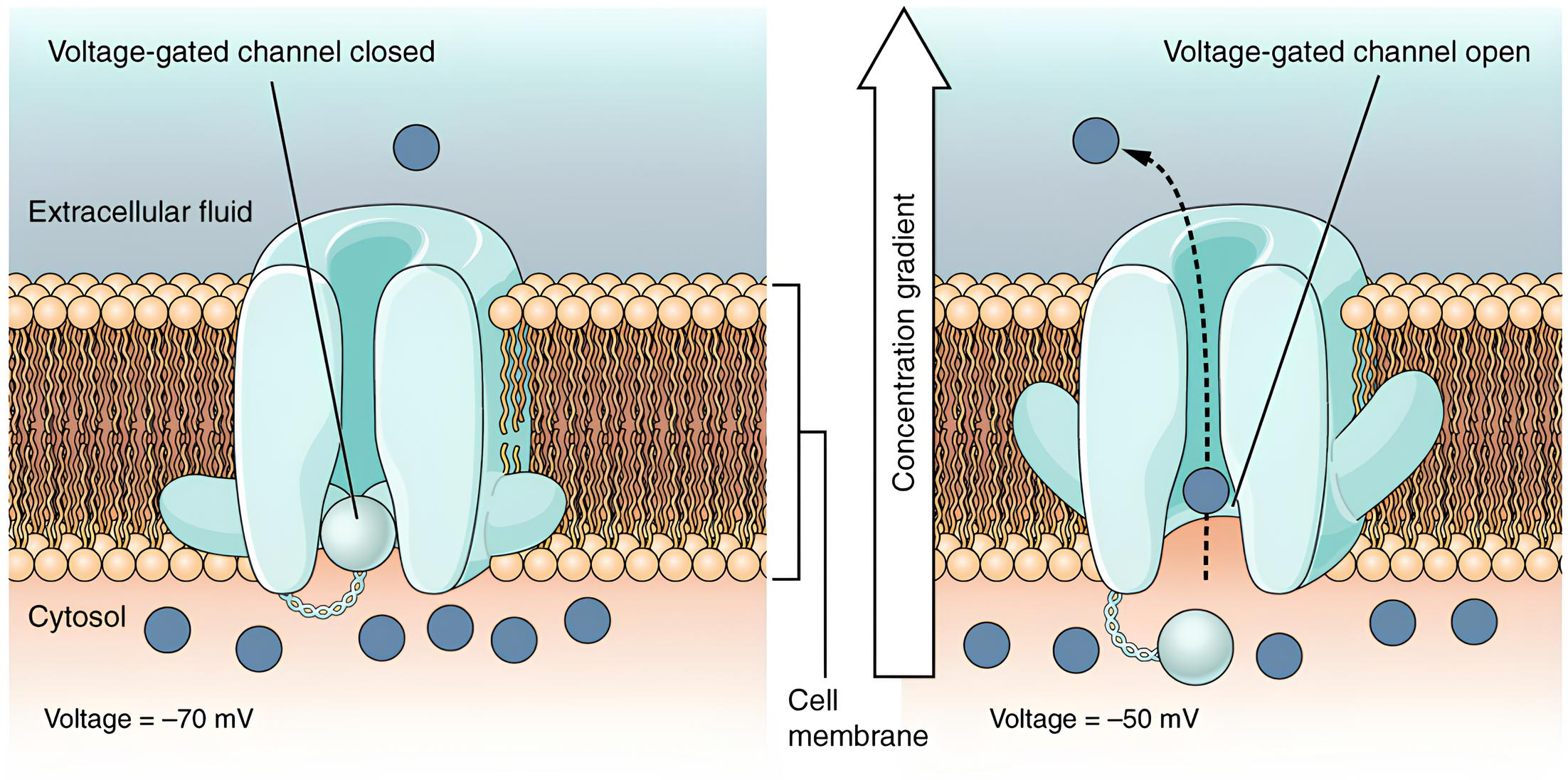
Right now, our neuron is basically a zombie. It’s just sitting there, leaking a bit of charge and generally being a bit of a slacker. No exciting messages, no action potentials, it’s like a town crier who’s decided to take an eternal nap. But fear not! Things are about to get much more interesting. We’re about to introduce the real heroes of the story: voltage-gated ion channels.

Photo from Neuroscience: Canadian 1st Edition

Now, let’s get a little mathematical here (don’t worry, we’ll keep it fun!). We need a function to describe how the membrane potential (\(V\)) changes over time (\(t\)) due to all that pesky leakage.

So, what kind of function would you use to describe something that decays gradually, like a deflating balloon? You guessed it! We need an exponential function, that classic workhorse of mathematical modeling.

Exponential functions look something like this:

input <- seq(0, 8, by = 0.01)

df <- data.table(input = input,
           `e^x` = exp(input),
           `-e^x` = -exp(input),
           `e^{-x}` = exp(-input),
           `-e^{-x}` = -exp(-input))

df <- melt(df, id.vars = "input")

ggplot(df, aes(input, value)) +
  facet_wrap(~ variable, labeller = "label_parsed", scales = "free_y") +
  geom_hline(yintercept = 0, linewidth = 1/2, 
             linetype = 2, col = "gray50") +
  geom_line(linewidth = 1, 
                col = "orange") +
  labs(x = "Input", y = "Output",
       title = "Exponential Function Dynamics")

Exponential Function and Common Variations. Here we see how changing a small detail in the original function (in this case a negative sign) can yield dramatically different behavior.

At first glance, we can see that the bottom variations of the exponential function (the ones with negative exponents) seem to behave more like a neuron should. They oscillate nicely, staying within a reasonable range. This function with the negative exponent, \(e^{-x}\), seems like a good starting point to describe how the membrane potential gradually returns to its resting state. It’s like watching a deflating balloon (slow and steady).

Customizing It Further: Tweaking the Decay Rate

Now, let’s get a little more creative! We can tweak this function to control how quickly the membrane potential returns to rest. Imagine it’s like adjusting the valve on a tire, you can control how fast the air leaks out.

We can do this by adding a “rate parameter” to our exponent. Instead of just \(e^{-x}\), we can use \(e^{-x \cdot \lambda}\). This \(\lambda\) value acts like a speed control for the decay. By changing \(\lambda\), we can adjust how quickly the membrane potential returns to its resting value. It’s like having a dial to control how fast the balloon deflates.

Let’s visualize this change and see how it affects the decay rate!

input <- seq(0, 10, by = 0.01)

df <- lapply(X = seq(0, 1.4, by = 0.2), function(x) {
  data.table(Input = input, 
             lambda = format(x, digits = 1, nsmall = 1),
             Output = exp(-input * x))
}) |> rbindlist()

ggplot(df, aes(Input, Output, color = ordered(lambda))) +
  geom_hline(yintercept = 0, linewidth = 1/2, 
             linetype = 2, col = "gray50") +
  geom_line(linewidth = 1) +
  labs(color = expression(lambda),
       y = expression(e^{-x*lambda}),
       title = expression("Rate Parameter ("*lambda*") on Output Dynamics"))

Effect of Rate Parameter on Function Dynamics. Here we see that by altering the rate parameter \(\lambda\) we can toy around with “how fast” our exponential function is returning to baseline.

Great! Now we need to give this function a little personality. Right now, it’s a bit generic. It always starts at 1 and decays towards 0. But what if we want to start at a different value? Or maybe we want it to decay towards a different value than 0?

No problem! We can easily customize this function.

First, let’s give it a starting point. We can add a multiplicative factor (let’s call it \(b\)) to the exponential function. This is like giving our function a “starting height”. Now, our function looks like this:

\[ b \cdot e^{-x \cdot \lambda} \]

Next, let’s give it a target value. We can add a linear factor (let’s call it \(a\)) to shift the entire curve up or down. This is like setting a new “ground level” for our function.

With these adjustments, our function now looks like this:

\[ a + b \cdot e^{-x \cdot \lambda} \]

This gives us much more flexibility! For example, if we set \(a\) to 0 and \(b\) to 1, we get our original function. It’s like having a basic template and then customizing it to fit our specific needs.

In fact, she did use it at the end. Photo from Frank Mariani in Cartoonist for Hire

But wait a minute! We’ve been doing all this math, and we haven’t even talked about neurons yet! What was the point of all this mental gymnastics? Well, it turns out that this seemingly random function has a very real biological meaning.

Let’s take a look at that equation again, but this time with some real neuron terms:

\[ V(t) = E_L + (V_0 - E_L) \cdot e^{-g_L \cdot t} \]

Now, this equation starts to make sense. It tells us how the membrane potential (\(V\)) changes over time (\(t\)). It’s like watching a movie of the membrane potential.

• \(V(t)\): This is the membrane potential at any given moment, the voltage across the cell membrane at that exact instant.
• \(E_L\): This is the “leak reversal potential”, the magical voltage where the leak channels are perfectly balanced. It’s like the “sweet spot” for the membrane, usually close to the resting membrane potential (around -70 mV). This is the value our function will try to get over time.
• \(V_0\): This is the starting point, the initial membrane potential at time \(t = 0\). It’s like the starting position in a race.
• \(g_L\): This is the “leak conductance”, a measure of how easily ions can leak through the membrane. Think of it as how wide the leaky faucet is open. A higher \(g_L\) means ions leak faster, and the membrane potential changes more quickly.
• \(e^{-g_L \cdot t}\): This is the exponential decay term, the engine that drives the change. It ensures that the membrane potential gradually approaches \(E_L\) over time, like a car slowly coming to a stop.

Now, let’s get a little more mathematical. If we want to express how the membrane potential changes over time, we need to find the “rate of change” of the membrane potential. In math terms, this is called the derivative.

Average Bayesically-Speaking reader going through the content on a typical blog post after I say “We’ll start with the basics”. Photo from Giphy

If we take the derivative of our previous equation (don’t worry, you don’t need to know the calculus!), we get something like this:

\[ \frac{d V}{d t} = -g_L \cdot (V_0 - E_L) \]

This equation tells us how fast the membrane potential is changing at any given moment.

Let’s break this down:

• \(\frac{d V}{d t}\): This fancy term represents the “rate of change” of the membrane potential. It tells us how quickly the voltage is rising or falling.
• \(g_L\): This is our old friend, the leak conductance. A higher \(g_L\) means the membrane is “more leaky”, and the membrane potential will change more rapidly.
• \((V_0 - E_L)\): This term represents the “driving force” for the leak current. The bigger the difference between the current potential and the leak reversal potential, the stronger the “urge” for the membrane potential to return to equilibrium. It’s like a ball rolling down a steep hill, the steeper the hill, the faster it rolls.

If the next plot, we’ll see the solution to this equation, an exponential decay curve. It’s like watching a ball rolling down a hill, it starts fast but gradually slows down as it approaches the bottom.

# Parameters
time <- seq(0, 50, 0.1) # Time vector

# Function to calculate membrane potential over time
membrane_potential <- function(time, V0, g_L, E_L) {
  V <- (V0 - E_L) * exp(-g_L * time) + E_L
  return(V)
}

# Starting membrane potentials
df <- lapply(c(-50,-60,-65,-68,-72,-75,-80,-90), function(x) {
           data.table(v = membrane_potential(time, V0 = x, g_L = 0.1, E_L = -70),
                      start_v = x,
                      time = time)
         }) |> 
  rbindlist()

# Create the plot using ggplot2
ggplot(df, aes(x = time, y = v, color = ordered(start_v))) +
  geom_line(linewidth = 1) +
  geom_hline(yintercept = -70, linetype = "dashed", color = "black", alpha = 0.7) + # Add E_L line
  labs(
    x = "Time (Arbitrary Units)",
    y = "Membrane Potential (mV)",
    title = "Membrane Potential Decay Due to Leak Current",
    color = "Starting Voltage (mV)"
  )

Membrane Potential and Leak Current. Here we can see that the membrane tends to return to its resting potential. This behavior is accomplished by the tweaks we made earlier to our exponential function.

For example, if we inject a small current that briefly changes the membrane potential to -60 mV, the membrane potential will decay back to -70 mV, following the equation.

Too Simple?

This simple model is important because it shows us how the membrane potential would behave passively, in the absence of any active processes. It explains how the resting membrane potential is maintained. However, it doesn’t explain the rapid, dramatic changes we see during an action potential. Our sleepy neuron is still just leaking and slowly returning to its resting state. It’s like watching paint dry (not exactly thrilling). We need something more to explain the neuron’s “shouting” behavior. That “something more” is the introduction of voltage-gated ion channels, which we’ll explore in the next section.

Okay, let’s add some simplified equations to represent the voltage-gated channels and incorporate them into our membrane potential equation.

Adding Voltage-Gated Channels: The Key to Excitation

Photo from Human Bio Media

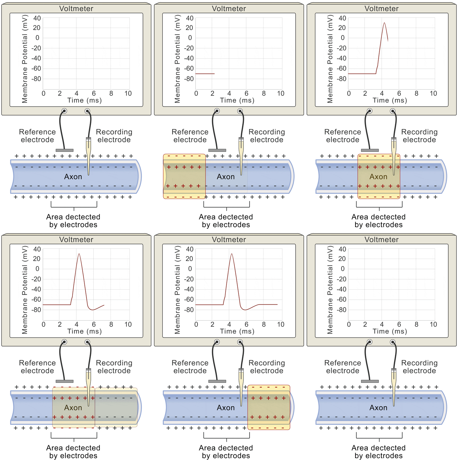
Okay, let’s get down to the nitty-gritty. How does this whole “voltage” thing actually work? Well, picture this: the change in voltage over time (basically how fast the voltage is shifting), is all about the flow of ions. You’ve got ions lazily leaking through the membrane (let’s call that the “lazy ion flow”), and then you’ve got the more exciting players: sodium, potassium, and even some other ions that like to join the party.

So, if we want to get fancy, we could say that the change in voltage over time, which we can write as \(\frac{dV}{dt}\) for all you math whizzes out there, is basically a sum of all these ion flows. We’ve got the lazy ion flow (\(I_L\)), the sodium party crashers (\(I_{Na}\)), the potassium crew (\(I_K\)), and any other surprise guests (\(I_{\text{other ions}}\)).

And if we want to put it all together in a fancy equation, we could say that:

\[ \frac{dV}{dt} = I_L + I_{Na} + I_K + \dots + I_{\text{other ions}} \]

So, now we’ve got this “leaky current” (\(I_L\)), which we can basically describe using that fancy equation \(-g_L \cdot (V_0 - E_L)\). But what about those exciting voltage-gated channels? How do we explain their contribution to the party? To figure that out, we need to dive deeper into the wild world of voltage-gated channel dynamics.

Remember our boring old passive membrane? It just kind of slumped back to its resting potential, like a deflated balloon. Well, our active neurons are a whole different story. They’ve got these amazing channels that open and close depending on the voltage, making the whole system much more exciting.

These channels, especially the sodium (\(Na^+\)) and potassium (\(K^+\)) channels, are the real stars of the show. They’re the ones that cause those dramatic swings in voltage during an action potential.

Sodium channels are like little gates. They have an “activation gate” (let’s call it gate \(m\)) that swings open around -55 mV. This is like the starting pistol for the race! Sodium ions flood into the cell, and the voltage skyrockets. But here’s the catch: these channels also have an “inactivation gate” (let’s call it gate \(h\)) that slams shut around +30 mV. It’s like the emergency brakes! This prevents the cell from exploding with too much sodium. And don’t worry, the inactivation gate eventually reopens when the cell calms down and returns to its resting potential (around -70 mV).

Sodium channel in an open state, illustrating its activation and inactivation gates. Photo from Human Bio Media

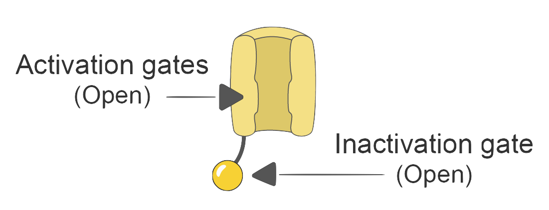
So, if we want to express the sodium current (\(I_{Na}\)) in all its glory, we could say that:

\[ I_{Na} = -g_{Na} \cdot m \cdot h \cdot (V_0 - E_{Na}) \]

Where:

• \(g_{Na}\): Sodium conductance (how easily sodium ions flow when channels are open).
• \(m\): Sodium activation gate (1 = open, 0 = closed).
• \(h\): Sodium inactivation gate (1 = open, 0 = closed). This gate introduces a delay and helps terminate the sodium current.
• \(E_{Na}\): Sodium reversal potential.

In contrast, potassium channels are a bit simpler. They only have one gate (let’s call it gate \(n\)), which acts like a slow-opening door. This gate starts to swing open around +30mV, allowing potassium ions to flood out of the cell. This outflow of positive charge helps bring the voltage back down to resting potential (a phase we call “repolarization”). But here’s the twist: this gate is a bit slow to close. It doesn’t fully shut until the voltage dips below -80 mV, which is even more negative than the resting potential. This creates a slight undershoot before the cell finally settles back down.

Potassium channel in an open state, with its only voltage-dependent gate. Photo from Human Bio Media

Just like we did with the sodium channels, we can express the potassium current (\(I_K\)) as the following:

\[ I_{K} = -g_{K} \cdot n \cdot (V_0 - E_{K}) \]

Where:

• \(g_K\): Potassium conductance.
• \(n\): Potassium activation gate (1 = open, 0 = closed).
• \(E_K\): Potassium reversal potential.

So now, our updated equation now looks like this:

\[ \begin{aligned} \frac{dV}{dt} = -&g_L \cdot (V - E_L) + \\ -&g_{Na} \cdot m \cdot h \cdot (V - E_{Na}) + \\ -&g_K \cdot n \cdot (V - E_K) \end{aligned} \]

To maintain clarity and focus on the core dynamics, we’ll use simplified “on/off” gating variables rather than the full Hodgkin-Huxley equations (which we can explore another time).

Simplified Gating: A Key Simplification

In the real world, these gating variables (m, h, and n) are described by some seriously complex equations in the full Hodgkin-Huxley model (see Yao et al. 2023). It’s like trying to understand the inner workings of a Swiss watch!

But for our simplified model, we’re going to take a shortcut. We’ll assume these gates simply snap open and shut based on the voltage. It’s like we’re replacing that intricate Swiss watch with a simple on/off switch. This simplification helps us grasp the fundamental principles of action potential generation without getting bogged down in a sea of equations.

With these additions, our model finally starts to show some exciting behavior! If the membrane potential reaches a certain “trigger point” (called the threshold), the sodium channels swing open wide (\(m\) = 1). It’s like a floodgate opening! Sodium ions rush into the cell, causing a rapid spike in voltage, that’s our action potential!

But then, the sodium inactivation gate slams shut (\(h\) = 0), and the potassium channels finally open their doors (\(n\) = 1). Potassium ions rush out of the cell, bringing the voltage back down to normal, that’s the “repolarization” phase.

Voltage-gated channels for sodium (Na⁺) and potassium (K⁺). ECF, extracellular fluid; ICF, intracellular fluid. Photo from Human Bio Media

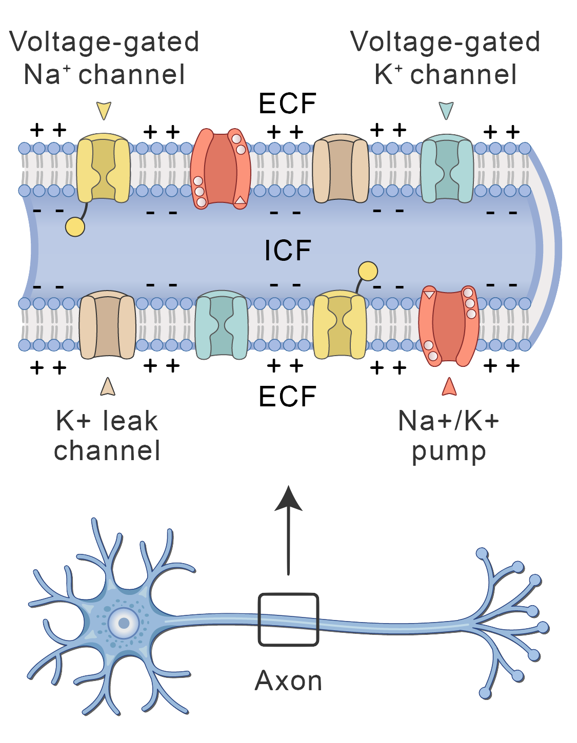
Now, let’s put this model into action! We’ll use something called the Euler method, which is basically a fancy way of numerically solving our equation. This will allow us to see how the membrane potential changes over time in response to a stimulus. It’s like running a simulation to see how our “neuron” behaves in the real world.

About the Hodgkin-Huxley Model

The Hodgkin-Huxley equations (see Hodgkin and Huxley 1939), developed in the mid-20th century, revolutionized our understanding of how neurons fire. These complex equations, initially derived from meticulous experiments on the giant squid axon, accurately model the intricate interplay of ion channels that generate the action potential.

Okay but, why it matters today? Well, for many reasons like:

• Foundation for modern neuroscience: The Hodgkin-Huxley model remains a cornerstone of computational neuroscience, providing a framework for understanding the electrical behavior of neurons.
• Drug development: Researchers use these equations to study the effects of drugs and toxins on neuronal activity, aiding in the development of new medications for neurological disorders.
• Artificial intelligence: Inspired by the Hodgkin-Huxley model, researchers are developing biologically realistic artificial neurons for use in neuromorphic computing, a promising area of artificial intelligence.

Simulating an Action Potential: Bringing the Model to Life

Alright, let’s get this show on the road! Now that we have our simplified mathematical model of the neuron, it’s time to bring it to life. We’ll use R, a powerful programming language, to simulate our model and watch how the membrane potential changes over time.

We’ll use a technique called the Euler method, which is basically like taking tiny little steps to solve our equation. It’s a bit like trying to reach a destination by taking a series of small hops instead of jumping straight there.

Average Bayesically-Speaking reader when is asked about their knowledge on voltage-gated channels. Photo from Wojak-Studio

Setting the Stage: Defining the Parameters

First, we need to define the parameters of our model. These parameters represent the properties of our neuron, such as how “leaky” the membrane is and the properties of the sodium and potassium channels. We also need to define the time step (dt), which determines how often we “take a picture” of the membrane potential during our simulation.

# Parameters
params <- list(
  g_L = 1, E_L = -70,   ## Leak Channels
  g_Na = 20, E_Na = 30, ## Sodium Channels
  g_K = 2, E_K = -90,   ## Potassium Channels
  dt = 0.001
)

Here:

• g_L: Leak conductance.
• E_L: Leak reversal potential (resting potential).
• g_Na: Sodium conductance.
• E_Na: Sodium reversal potential.
• g_K: Potassium conductance.
• E_K: Potassium reversal potential.
• dt: Time step (0.001 ms).

The Sodium Activation Gate: The On/Off Switch

The sodium activation gate (m) is like the “on” switch for sodium channels. When the membrane potential (V_prev) reaches a critical point, around -55 mV, this gate swings open instantly, allowing sodium ions to flood in. It’s like someone yelling “Go!” at a starting line.

In our simplified model, we’re making a big assumption: this gate is an all-or-nothing switch. Either it’s completely open (m becomes 1) or completely closed (m is 0). This is a simplification, but it helps us capture the essence of the rapid rise of the action potential.

update_m <- function(V_prev) {
  ifelse(V_prev > -55, 1, 0)
}

This function takes the previous membrane potential (V_prev) as input and tells us whether the sodium activation gate is open or closed.

The Sodium Inactivation Gate: The Emergency Brake

The sodium inactivation gate (h) is like the emergency brake for the sodium channels. It starts open (h = 1) at rest, but when the membrane depolarizes and sodium channels open wide (m = 1), this gate slowly starts to close (h transitions towards 0). This is crucial to prevent a runaway influx of sodium.

However, the inactivation gate only starts to close when the membrane potential is sufficiently positive (around +20 mV). It’s like the brake only engages when the car is going fast enough.

Conversely, when the membrane repolarizes and the sodium channels close (m = 0), the inactivation gate slowly reopens (h transitions towards 1). But this recovery only happens when the membrane potential is sufficiently negative (around -70 mV). It’s like the brake only releases when the car has slowed down significantly.

This conditional behavior is implemented in the following function:

update_h <- function(m_current, V_prev, h_prev) {
  ifelse(
    test = m_current == 1 & V_prev >= 20, 
    yes = 0, 
    no = ifelse(
      test = m_current == 0 & V_prev <= -70, 
      yes = 1, 
      no = h_prev
    )
  )
}

This function takes the current value of m (m_current), the previous membrane potential (V_prev), and the previous value of h (h_prev) as inputs and returns the updated value of h.

The Potassium Activation Gate: The Slow and Steady Door

The potassium activation gate (n) is like a slow-opening door. It starts to open when the membrane potential reaches a sufficiently positive value (around +20 mV). But unlike the sodium gate, it’s a bit sluggish.

There’s also a bit of “hysteresis” here. This means that the potassium gate only closes when the membrane potential becomes extremely negative (around -80 mV) and it was already open in the previous time step. It’s like the door is reluctant to close once it’s been opened. This hysteresis ensures that the membrane repolarizes completely before the potassium channels fully close.

update_n <- function(V_prev, n_prev) {
  ifelse(
    test = V_prev >= 20, 
    yes = 1, 
    no = ifelse(
      test = V_prev <= -80 & n_prev == 1, 
      yes = 0, 
      no = n_prev
    )
  )
}

This function takes the previous membrane potential (V_prev) and the previous value of n (n_prev) as input and returns the updated value of n.

Calculating the Ion Flows: The Grand Finale

This function calculates the flow of ions across the membrane. We have three main players:

• The Leaky Current: This is the “background” current, where ions slowly leak through the membrane.
• The Sodium Current: This is where the action happens! It’s influenced by the sodium activation gate (m) and the inactivation gate (h).
• The Potassium Current: This current is controlled by the potassium activation gate (n).

To calculate each current, we use a simple formula: \(I = g \cdot (V - E)\). It’s like calculating the flow of water through a pipe, where \(g\) represents the size of the pipe, \(V\) is the pressure difference, and \(E\) is a kind of “equilibrium point.”

calculate_currents <- 
  function(V_prev, m, h, n, params) {
    
  l_current <- -params$g_L * (V_prev - params$E_L)
  na_current <- -params$g_Na * m * h * (V_prev - params$E_Na)
  k_current <- -params$g_K * n * (V_prev - params$E_K)
  
  output <- list(l_current = l_current, 
                 na_current = na_current, 
                 k_current = k_current)
  
  return(output)
}

This function takes the previous membrane potential (V_prev), the gating variables (m, h, n), and the parameters (params) as input and returns a list containing the calculated currents.

Simulating Neurons in Action: Bringing it All Together!

This is the grand finale! This function brings all the pieces together to simulate how our neuron actually behaves. It takes the model parameters, a time vector (which tells us how long to run the simulation), and a stimulus current (like an external input to the neuron) as input.

Then, it iterates through each time step, updating the gating variables (those pesky “m,” “h,” and “n” gates) and calculating how the membrane potential changes using the Euler method. It’s like watching a movie frame-by-frame, seeing how the neuron responds to the different inputs.

simulate_ap <- function(params, time, stimulus_current) {
  n <- length(time)
  V <- rep(params$E_L, n) # Initialize Membrane potential
  m <- numeric(n) # Initialize Sodium Activation
  h <- rep(1, n) # Initialize Sodium Inactivation
  n_inf <- numeric(n) # Initialize Potassium Activation
  l_current <- numeric(n) # Initialize Leak Current
  na_current <- numeric(n) # Initialize Sodium Current
  k_current <- numeric(n) # Initialize Potassium Current
  
  for (i in 2:n) {
    ## Updates the state of each channel's gates
    m[i] <- update_m(V[i - 1])
    h[i] <- update_h(m[i], V[i - 1], h[i - 1])
    n_inf[i] <- update_n(V[i - 1], n_inf[i - 1])
    
    ## Compute the current 
    currents <- calculate_currents(
      V_prev = V[i - 1], 
      m = m[i], 
      h = h[i], 
      n = n_inf[i], 
      params = params
    )
    
    l_current[i] <- currents$l_current
    na_current[i] <- currents$na_current
    k_current[i] <- currents$k_current
    
    ## Sum each current contribution to the overall voltage change
    dVdt <- 
      l_current[i] + 
      na_current[i] + 
      k_current[i] + 
      stimulus_current[i]
    
    ## Update the Voltage based on current net flow
    V[i] <- 
      V[i - 1] + dVdt * params$dt
  }
  
  output <- data.table(Time = time, Voltage = V)
  return(output)
}

This function gets the party started! It initializes the membrane potential and all those gating variables (“m,” “h,” and “n”) to their starting values. Then, it enters a loop, stepping through time and updating these variables at each step. It’s like watching a movie play out frame-by-frame, observing how the membrane potential changes in response to the shifting currents.

Now, let’s run this simulation and see what happens! We’ll visualize the results to get a better understanding of how the neuron behaves.

# Simulation time
time <- seq(0, 8, by = params$dt)

# Stimulus
stimulus_current <- numeric(length(time))
stimulus_current[time > 2 & time < 2.5] <- 50

# Run the simulation
df <- simulate_ap(params, time, stimulus_current)

# Plotting
ggplot(df, aes(Time, Voltage)) +
  geom_hline(yintercept = -70, linewidth = 1/2, linetype = 2, col = "gray50") +
  geom_line(linewidth = 1, color = "orange") +
  labs(x = "Time (ms)", y = "Membrane Potential (mV)", title = "Simplified Action Potential Model")

Simplified Action Potential Model. Here we can see that after taking into account each contribution to the overall voltage dynamics over time (based on net current flow), we can see something more alike to a real action potential curve.

Tweaking the Knobs: Sensitivity Analysis

Now that we have our neuron simulation up and running, let’s see what happens when we start tinkering with the settings. This is called sensitivity analysis. We’ll systematically change one parameter at a time and see how it affects the neuron’s behavior. It’s like tweaking the knobs on a radio to see how it changes the sound.

This analysis is crucial for understanding how our model works and figuring out which parameters have the biggest impact on the action potential. It’s like trying to figure out which ingredients are most important for baking the perfect cake.

To make this process easier, we’ll create a special function called sensitivity_analysis. This function takes the model parameters, the time vector, the stimulus current, the name of the parameter we want to change (param_name), and a list of values we want to test for that parameter (values) as input. It then runs the simulation for each value in the list, stores the results, and combines them all into a single, organized data frame.

sensitivity_analysis <- 
  function(params, time, stimulus_current, param_name, values) {
  
    results <- vector(mode = "list")
    
    for (value in values) {
      # Modify the parameter value
      modified_params <- params
      modified_params[[param_name]] <- value 
      
      # Run the simulation
      df <- simulate_ap(modified_params, time, stimulus_current) 
      
      # Add a column to track the parameter value
      df$ParameterValue <- value
      
      # Store the results
      results[[as.character(value)]] <- df
    }
    
    output <- rbindlist(results)
    return(output) # Combine all data.tables into one
}

Inside the function, we do the following:

1. Create an empty list: We create an empty list called results to store the output of each simulation. Think of it as an empty box to store all our simulation results.
2. Loop through the values: We loop through each value in the list of values we want to test. It’s like trying different settings on a machine one by one.
3. Make a copy: We create a copy of our original parameters called modified_params. This is crucial to avoid messing up the original settings.
4. Tweak the parameter: We modify the specific parameter (param_name) in our modified_params copy to the current value from our list.
5. Run the simulation: We run our simulate_ap function with these modified parameters to see how the neuron behaves.
6. Add a label: We add a new column called ParameterValue to the results to keep track of which parameter value we used for that simulation. It’s like labeling each experiment.
7. Store the results: We store the results of this simulation in our results list, using the parameter value as a label for easy reference.
8. Combine the results: Finally, we use a special function called rbindlist to neatly combine all the individual data frames in our results list into one big data frame. This gives us a complete overview of how the neuron behaves with different parameter settings.

The Plotting Function: Seeing the Results

Now, let’s visualize our results! We’ll create a special function called plot_sensitivity to do this. This function takes the combined results data frame and the name of the parameter we were analyzing as input. It then generates a plot that shows how the membrane potential changes over time for each of the parameter values we tested. It’s like creating a visual story of how the neuron behaves under different conditions.

plot_sensitivity <- function(results, param_name) {
  ggplot(results, aes(Time, Voltage, color = factor(ParameterValue))) +
    geom_hline(yintercept = -70, linewidth = 1/2, linetype = 2, col = "gray50") +
    geom_line(linewidth = 1) +
    labs(x = "Time (ms)", y = "Membrane Potential (mV)", 
         title = scales::label_parse()(paste("Sensitivity~Analysis~of~", param_name))) +
    scale_color_ordinal(name = scales::label_parse()(param_name))
}

This function creates a line plot using ggplot2, where the x-axis represents time, the y-axis represents the membrane potential, and different colors represent different values of the varied parameter. The factor() function is used to treat the ParameterValue as a categorical variable, ensuring that each value gets a distinct color in the plot.

Your face after I told you that we’re going to see the basics and it turned out not so basic after all. Photo from Pinteres

Setting the Stage for Simulations

Before we dive into the nitty-gritty of sensitivity analysis, we need to set the stage for our simulations.

• Time: We define the simulation time, which tells us how long to run the experiment. We’ll run the simulation from 0 to 8 milliseconds (ms).
• Time Step: We need to decide how often we “take a picture” of the membrane potential. This is determined by the dt parameter in our params list.
• Stimulus: We’ll create a brief stimulus current, like a little jolt of electricity, that’s applied between 0.5 and 1.0 milliseconds.

# Simulation time and stimulus
time <- seq(0, 6, by = params$dt)
stimulus_current <- numeric(length = length(time))
stimulus_current[time > 0.5 & time < 1.0] <- 50

Assessing the Effect of Sodium Conductance (\(g_{Na}\)): Turning Up the Heat

Now, let’s see what happens when we tweak the sodium conductance (\(g_{Na}\)). This is like adjusting the heat on a stove.

# Run sensitivity analysis for g_Na
gna_values <- c(9.5, 10, 12, 15, 20)

gna_results <- sensitivity_analysis(params, time, stimulus_current, "g_Na", gna_values)

plot_sensitivity(gna_results, "g[Na]")

Effect of Sodium Conductance in Potential Dynamics. Here we can see the overall effect of changing the sodium conductance on membrane potential dynamics.

By running our sensitivity_analysis function and then plotting the results, we can clearly see how changing \(g_{Na}\) affects the action potential. It’s like watching how turning up the heat affects how quickly water boils. As expected, increasing \(g_{Na}\) makes the depolarization much faster and more dramatic.

Assessing the Effect of Potassium Conductance (\(g_{K}\)): Controlling the Cool-Down

Next, let’s see how changing the potassium conductance (\(g_{K}\)) affects things. This is like adjusting the thermostat, it controls the cool-down period.

# Run sensitivity analysis for g_K
gk_values <- c(1, 2, 5, 10)

gk_results <- sensitivity_analysis(params, time, stimulus_current, "g_K", gk_values)

plot_sensitivity(gk_results, "g[K]")

Effect of Potassium Conductance in Potential Dynamics. Here we can see the overall effect of changing the potassium conductance on membrane potential dynamics.

Again, using our handy functions, we can easily see how \(g_{K}\) impacts the action potential. Increasing \(g_{K}\) makes the repolarization phase much faster and more pronounced. It’s like adding more ice to a hot drink, it cools down much quicker. This structured approach allows us to efficiently explore how different parameters affect our model and gain a deeper understanding of its dynamics.

So, You Think You Know How a Neuron Fires? Think Again!

Okay, let’s be honest, this “action potential” business is a bit overhyped. It’s basically just a fancy term for a sudden influx of sodium ions followed by a swift efflux of potassium. Really, who needs all those fancy textbooks and intimidating equations? (Kidding! We need them).

Our little model here? Yeah, it’s basically a “neuron for beginners”. We stripped it down to the essentials, ignoring the nitty-gritty details like how ion channels actually open and close and the subtle ways different potassium channels interact. Who needs that level of detail, right?¹

¹ In fact we do! But that much level of detail is reserved for another blog post

Now, let’s get real for a second. Real neurons? They’re not this simple. Oh no. They have a whole zoo of ion channels, each with its own quirks and preferences for voltage (Drukarch and Wilhelmus 2023). Sodium channels? Potassium channels? Please, it’s more like a neurochemical orchestra! And don’t even get me started on the calcium-dependent potassium channels…

But hey, our little “dumbed-down” neuron serves a purpose. It’s like, the “Cliff’s Notes” of neurophysiology. You get the main idea, you understand the basic principles of membrane excitability. And that, my friends, is enough to impress at your next cocktail party.

Now, let’s talk about drugs. Oh boy, drugs. You know, those pesky little molecules that interfere with neuronal signaling? Well, guess what? They love to target these ion channels. Lidocaine? Blocks sodium channels, basically shutting down the neuron. Potassium channel blockers? Well, let’s just say they can make neurons go wild. Our model? It can predict these effects, to a certain extent. Of course, it’s not exactly a perfect predictor of pharmacological outcomes. But hey, it’s a start.

And finally, let’s talk about the big picture. Communication. You know, how your brain actually does stuff? Well, it all starts with these action potentials. They’re like, the brain’s version of Morse code. But instead of dots and dashes, it’s a symphony of electrical impulses, traveling along axons and triggering the release of neurotransmitters. And our little model? It gives us a glimpse into this mysterious world of neuronal chatter.

Motor Neurons (Multipolar) with many Processes (mostly Dendrites). Photo from Neurology Advisor

Hasta la Vista Baby

So, there you have it. Our “simplified” action potential model. Not exactly a perfect mirror of reality, but hey, it’s a good start. Now go forth and explore the wonders of neuroscience! Dive deeper into the hows and whys of ion channel behavior, uncover the secrets of synaptic transmission, and maybe even contribute to the next big breakthrough in neuroscience! The human brain is an incredibly complex machine, and understanding its workings is a journey of endless fascination.

Just remember, this is just the tip of the iceberg. Real neurons are far more sophisticated than our little model. They’re a tornado of activity, a symphony of ions, and a constant dance of electrical signals. But hey, at least now you have a basic understanding of how these amazing cells work.

Disclaimer: This model is for entertainment purposes only. Please do not attempt to perform any neurological procedures based on the information presented here (or maybe try it, but don’t mention my name).

Now go forth and amaze your friends with your newfound knowledge of neurophysiology. Just don’t get carried away and start diagnosing everyone with “abnormal neuronal activity”. And most importantly, remember to have fun! Neuroscience is a fascinating field, and there’s always something new to learn.

References

Drukarch, Benjamin, and Micha MM Wilhelmus. 2023. “Thinking about the Action Potential: The Nerve Signal as a Window to the Physical Principles Guiding Neuronal Excitability.” Frontiers in Cellular Neuroscience 17: 1232020.

Hodgkin, Alan L, and Andrew F Huxley. 1939. “Action Potentials Recorded from Inside a Nerve Fibre.” Nature 144 (3651): 710–11.

Rubin, Devon I. 2021. “Basics of Neurophysiology.” Clinical Neurophysiology, 9.

Yao, Wei, Yingchen Li, Zhihao Ou, Mingzhu Sun, Qiongxu Ma, and Guanghong Ding. 2023. “Dynamic Analysis of Neural Signal Based on Hodgkin–Huxley Model.” Mathematical Methods in the Applied Sciences 46 (4): 4676–87.